The End Of Knowledge - Vault 5/54 - CVPR - 2020 - BSP-Net: Generating Compact Meshes via Binary Space Partitioning

graph LR classDef bspnet fill:#f9d4d4, font-weight:bold, font-size:14px classDef existing fill:#d4f9d4, font-weight:bold, font-size:14px classDef comparison fill:#d4d4f9, font-weight:bold, font-size:14px classDef components fill:#f9f9d4, font-weight:bold, font-size:14px A[BSP-Net: Generating Compact
Meshes via Binary
Space Partitioning] --> B[BSPNet: compact watertight meshes 1] A --> C[Existing: warp or implicit 2] C --> D[Implicit: marching cubes, too many 3] B --> E[BSPNet: compact, sharp, curved 4] B --> F[Key: BSP trees, planes 5] B --> G[Process: intersections, convex, union 6] A --> H[Network: BSP tree components 7] H --> I[Input: voxel or image 8] H --> J[MLP: feature to plane 9] H --> K[Training: points, sign distances 10] H --> L[Connections: binary matrix 11] H --> M[Output: weighted sum, mean 12] A --> N[Training: two-stage, losses 13] N --> O[Stage 1: continuous, change 14] N --> P[Stage 2: binary, mean 15] A --> Q[2D: images, convex parts 16] A --> R[Segmentations: convex level 17] A --> S[Comparison: better reconstruction, segmentation 18] A --> T[3D: manual, semantic parts 19] A --> U[Decoder: single-view reconstruction 20] A --> V[Comparison: comparable, fewer polygons 21] A --> W[CVXNet: convex, BSPNet low-poly 22] A --> X[Code: available on GitHub 23] class B,E,F,G bspnet class C,D existing class H,I,J,K,L,M components class S,V comparison

Resume:

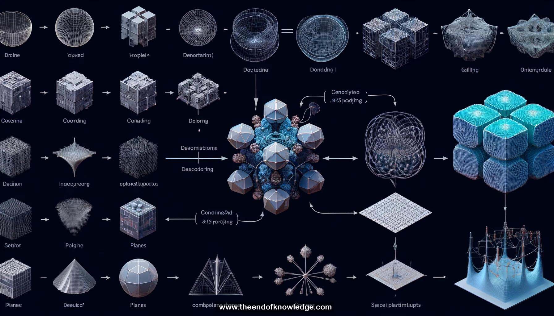
1.- BSPNet: generates compact, low-poly, watertight meshes using binary space partitioning.

2.- Existing methods: warp template meshes or use implicit functions, resulting in non-compact meshes.

3.- Implicit methods: require marching cubes, producing meshes with too many polygons.

4.- BSPNet advantages: compact output meshes with few primitives, reproducing sharp details and approximating curved boundaries.

5.- Key idea: derived from binary space partitioning trees using oriented planes and connections.

6.- Process: compute intersections within groups to obtain convex shapes, then union them.

7.- Network design: each component represents a part of the BSP tree.

8.- Input: voxel model or image, encoded to get feature code.

9.- MLP: maps feature code to plane parameters (leaf nodes in BSP tree).

10.- Training: sample points in space, calculate sign distances.

11.- Connections: represented by a trainable binary matrix.

12.- Output shape: obtained by weighted sum or mean pooling of convex shapes.

13.- Training process: two-stage approach with reconstruction loss and tree-structuring losses.

14.- Stage 1: train network with continuous weights, change connections.

15.- Stage 2: binarize connection weights, replace weighted sum with mean pooling.

16.- 2D toy experiment: network reconstructs images as combinations of convex parts.

17.- Shape segmentations and correspondences: found at the convex level.

18.- Comparison: better reconstruction quality and segmentation results than other decomposition methods.

19.- 3D case: manual grouping of convexes into semantic parts, visualizing correspondences.

20.- Differentiable 3D decoder: pairs with image encoder for single-view reconstruction.

21.- Comparison with state-of-the-art methods: comparable performance with fewer vertices and triangles.

22.- CVXNet: another convex decomposition method, but BSPNet targets low-poly reconstruction with dynamic convex numbers.

23.- Source code: available on GitHub.

Knowledge Vault built byDavid Vivancos 2024